Plot a rater_fit object
# S3 method for class 'rater_fit'
plot(
  x,
  pars = "theta",
  prob = 0.9,
  rater_index = NULL,
  item_index = NULL,
  theta_plot_type = "matrix",
  ...
)
Arguments
- x
An object of class
rater_fit.- pars
A length one character vector specifying the parameter to plot. By default
"theta".- prob
The coverage of the credible intervals shown in the
"pi"plot. If not plotting pi this argument will be ignored. By default0.9.- rater_index
The indexes of the raters shown in the
"thetaplot. If not plotting theta this argument will be ignored. By defaultNULLwhich means that all raters will be plotted.- item_index
The indexes of the items shown in the class probabilities plot. If not plotting the class probabilities this argument will be ignored. By default
NULLwhich means that all items will be plotted. This argument is particularly useful to focus the subset of items with substantial uncertainty in their class assignments.- theta_plot_type
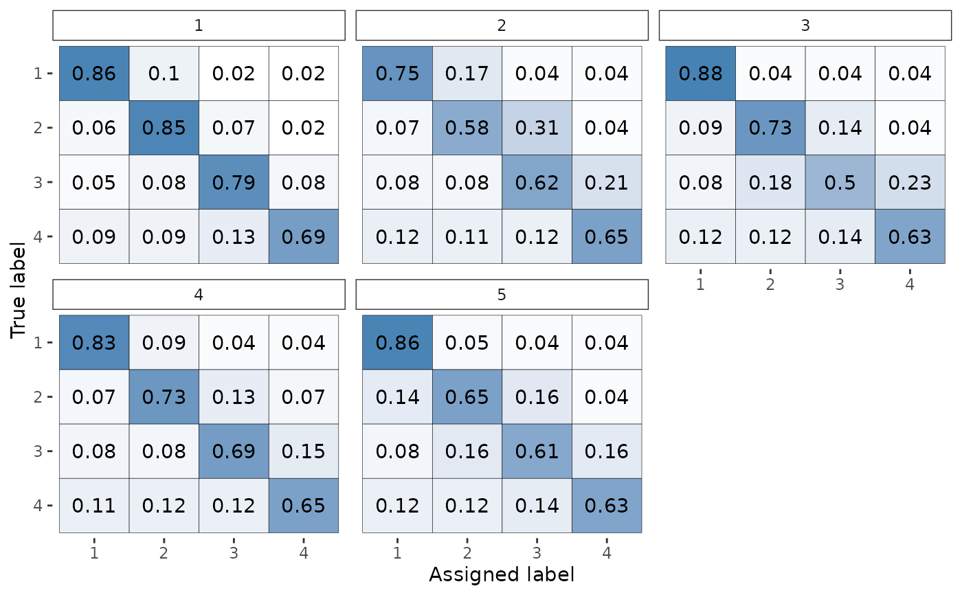
The type of plot of the "theta" parameter. Can be either
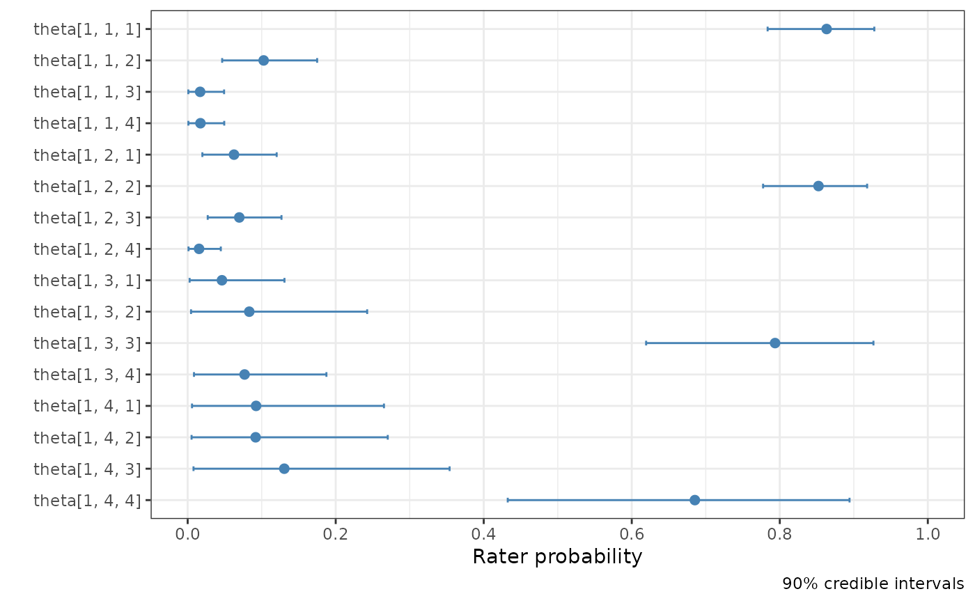
"matrix"or"points". If"matrix"(the default) the plot will show the point estimates of the individual rater error matrices, visualised as tile plots. If"points", the elements of the theta parameter will be displayed as points, with associated credible intervals. Overall, the"matrix"type is likely more intuitive, but the"points"type can also visualise the uncertainty in the parameter estimates.- ...
Other arguments.
Value
A ggplot2 object.
Details
The use of pars to refer to only one parameter is for backwards
compatibility and consistency with the rest of the interface.
Examples
# \donttest{
fit <- rater(anesthesia, "dawid_skene")
#>
#> SAMPLING FOR MODEL 'dawid_skene' NOW (CHAIN 1).
#> Chain 1:
#> Chain 1: Gradient evaluation took 9.2e-05 seconds
#> Chain 1: 1000 transitions using 10 leapfrog steps per transition would take 0.92 seconds.
#> Chain 1: Adjust your expectations accordingly!
#> Chain 1:
#> Chain 1:
#> Chain 1: Iteration: 1 / 2000 [ 0%] (Warmup)
#> Chain 1: Iteration: 200 / 2000 [ 10%] (Warmup)
#> Chain 1: Iteration: 400 / 2000 [ 20%] (Warmup)
#> Chain 1: Iteration: 600 / 2000 [ 30%] (Warmup)
#> Chain 1: Iteration: 800 / 2000 [ 40%] (Warmup)
#> Chain 1: Iteration: 1000 / 2000 [ 50%] (Warmup)
#> Chain 1: Iteration: 1001 / 2000 [ 50%] (Sampling)
#> Chain 1: Iteration: 1200 / 2000 [ 60%] (Sampling)
#> Chain 1: Iteration: 1400 / 2000 [ 70%] (Sampling)
#> Chain 1: Iteration: 1600 / 2000 [ 80%] (Sampling)
#> Chain 1: Iteration: 1800 / 2000 [ 90%] (Sampling)
#> Chain 1: Iteration: 2000 / 2000 [100%] (Sampling)
#> Chain 1:
#> Chain 1: Elapsed Time: 1.282 seconds (Warm-up)
#> Chain 1: 1.359 seconds (Sampling)
#> Chain 1: 2.641 seconds (Total)
#> Chain 1:
#>
#> SAMPLING FOR MODEL 'dawid_skene' NOW (CHAIN 2).
#> Chain 2:
#> Chain 2: Gradient evaluation took 8.7e-05 seconds
#> Chain 2: 1000 transitions using 10 leapfrog steps per transition would take 0.87 seconds.
#> Chain 2: Adjust your expectations accordingly!
#> Chain 2:
#> Chain 2:
#> Chain 2: Iteration: 1 / 2000 [ 0%] (Warmup)
#> Chain 2: Iteration: 200 / 2000 [ 10%] (Warmup)
#> Chain 2: Iteration: 400 / 2000 [ 20%] (Warmup)
#> Chain 2: Iteration: 600 / 2000 [ 30%] (Warmup)
#> Chain 2: Iteration: 800 / 2000 [ 40%] (Warmup)
#> Chain 2: Iteration: 1000 / 2000 [ 50%] (Warmup)
#> Chain 2: Iteration: 1001 / 2000 [ 50%] (Sampling)
#> Chain 2: Iteration: 1200 / 2000 [ 60%] (Sampling)
#> Chain 2: Iteration: 1400 / 2000 [ 70%] (Sampling)
#> Chain 2: Iteration: 1600 / 2000 [ 80%] (Sampling)
#> Chain 2: Iteration: 1800 / 2000 [ 90%] (Sampling)
#> Chain 2: Iteration: 2000 / 2000 [100%] (Sampling)
#> Chain 2:
#> Chain 2: Elapsed Time: 1.261 seconds (Warm-up)
#> Chain 2: 1.259 seconds (Sampling)
#> Chain 2: 2.52 seconds (Total)
#> Chain 2:
#>
#> SAMPLING FOR MODEL 'dawid_skene' NOW (CHAIN 3).
#> Chain 3:
#> Chain 3: Gradient evaluation took 8.6e-05 seconds
#> Chain 3: 1000 transitions using 10 leapfrog steps per transition would take 0.86 seconds.
#> Chain 3: Adjust your expectations accordingly!
#> Chain 3:
#> Chain 3:
#> Chain 3: Iteration: 1 / 2000 [ 0%] (Warmup)
#> Chain 3: Iteration: 200 / 2000 [ 10%] (Warmup)
#> Chain 3: Iteration: 400 / 2000 [ 20%] (Warmup)
#> Chain 3: Iteration: 600 / 2000 [ 30%] (Warmup)
#> Chain 3: Iteration: 800 / 2000 [ 40%] (Warmup)
#> Chain 3: Iteration: 1000 / 2000 [ 50%] (Warmup)
#> Chain 3: Iteration: 1001 / 2000 [ 50%] (Sampling)
#> Chain 3: Iteration: 1200 / 2000 [ 60%] (Sampling)
#> Chain 3: Iteration: 1400 / 2000 [ 70%] (Sampling)
#> Chain 3: Iteration: 1600 / 2000 [ 80%] (Sampling)
#> Chain 3: Iteration: 1800 / 2000 [ 90%] (Sampling)
#> Chain 3: Iteration: 2000 / 2000 [100%] (Sampling)
#> Chain 3:
#> Chain 3: Elapsed Time: 1.391 seconds (Warm-up)
#> Chain 3: 1.336 seconds (Sampling)
#> Chain 3: 2.727 seconds (Total)
#> Chain 3:
#>
#> SAMPLING FOR MODEL 'dawid_skene' NOW (CHAIN 4).
#> Chain 4:
#> Chain 4: Gradient evaluation took 8.6e-05 seconds
#> Chain 4: 1000 transitions using 10 leapfrog steps per transition would take 0.86 seconds.
#> Chain 4: Adjust your expectations accordingly!
#> Chain 4:
#> Chain 4:
#> Chain 4: Iteration: 1 / 2000 [ 0%] (Warmup)
#> Chain 4: Iteration: 200 / 2000 [ 10%] (Warmup)
#> Chain 4: Iteration: 400 / 2000 [ 20%] (Warmup)
#> Chain 4: Iteration: 600 / 2000 [ 30%] (Warmup)
#> Chain 4: Iteration: 800 / 2000 [ 40%] (Warmup)
#> Chain 4: Iteration: 1000 / 2000 [ 50%] (Warmup)
#> Chain 4: Iteration: 1001 / 2000 [ 50%] (Sampling)
#> Chain 4: Iteration: 1200 / 2000 [ 60%] (Sampling)
#> Chain 4: Iteration: 1400 / 2000 [ 70%] (Sampling)
#> Chain 4: Iteration: 1600 / 2000 [ 80%] (Sampling)
#> Chain 4: Iteration: 1800 / 2000 [ 90%] (Sampling)
#> Chain 4: Iteration: 2000 / 2000 [100%] (Sampling)
#> Chain 4:
#> Chain 4: Elapsed Time: 1.269 seconds (Warm-up)
#> Chain 4: 1.372 seconds (Sampling)
#> Chain 4: 2.641 seconds (Total)
#> Chain 4:
# By default will just plot the theta plot
plot(fit)
 # Select which parameter to plot.
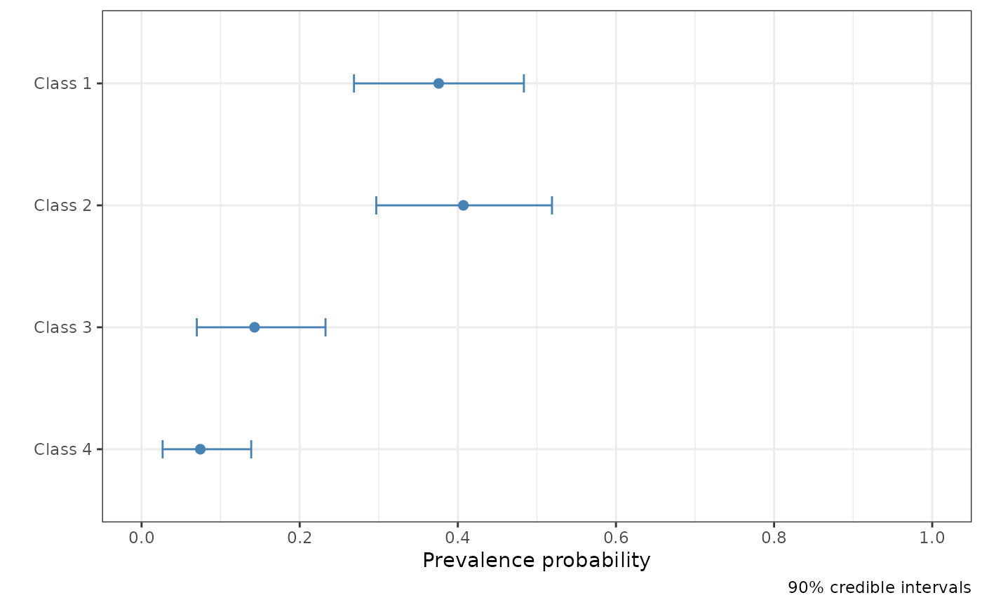
plot(fit, pars = "pi")
# Select which parameter to plot.
plot(fit, pars = "pi")
 # Plot the theta parameter for rater 1, showing uncertainty.
plot(fit, pars = "theta", theta_plot_type = "points", rater_index = 1)
# Plot the theta parameter for rater 1, showing uncertainty.
plot(fit, pars = "theta", theta_plot_type = "points", rater_index = 1)
 # }
# }